

Introduction for the approach
What is Image Processing?
Image processing is a method to perform some operations on an image, in order to get an enhanced image or to extract some useful information from it.
What is deep learning in image processing?
Deep learning is a type of machine learning in which a model learns to perform classification tasks directly from images, text or sound. Deep learning is usually implemented using neural network architecture. The term deep refers to the number of layers in the network—the more the layers, the deeper the network
What is CNN?
A Convolutional neural network (CNN) is a neural network that has one or more convolutional layers.
Those are used mainly for image processing, classification, segmentation and also for other auto correlated data.

A Convolutional Neural Network is a Deep Learning algorithm which can take in an input image, assign importance recognise differences in various angles that helps image to show its specialities one to another.
Why Python?
Finally Deep Learning is becoming a very popular subset of machine learning. Due to its high level of performance across many types of data.
A great way to use deep learning to classify images is to build a convolutional neural network (CNN). The Keras library in Python makes it pretty simple to build a CNN.
Dataset
Dataset includes exactly 6899 images as jpg. It has images categorised into folders by animal, cat, dog, car, air-plane, flower, fruit, motorbike, person.
Why do we use grayscale and not RGB/Colour Images?
All the colourful images are created by RGB values ( by combining different levels of Red, Blue, And Green colours). In this case having multiple colour channels is that we have huge volumes of data to work with which makes the process computationally intensive.
By using grayscale images on the role of CNN will reduce the images into a form that is easier to process, without losing features critical towards a good prediction. This is important when we need to make the algorithm scalable to massive datasets.
What are convolutions?
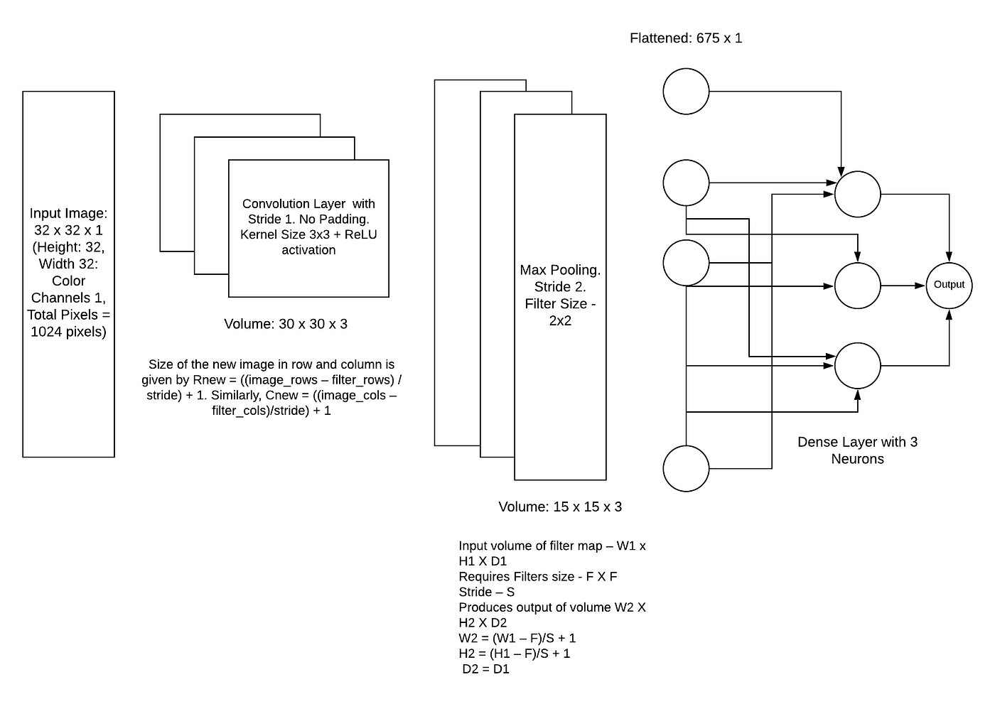
We understand that the training data consists of grayscale images which will be an input to the convolution layer to extract features. The convolution layer consists of one or more Kernels with different weights that are used to extract features from the input image. Say in the example above we are working with a Kernel (K) of size 3 x 3 x 1 (x 1 because we have one color channel in the input image), having weights outlined below.
Kernel/Filter, K =
1  0  1
0  1  0
1  0  1
When we slide the Kernel over the input image (say the values in the input image are grayscale intensities) based on the weights of the Kernel we end up calculating features for different pixels based on their surrounding/neighboring pixel values.
Why ReLU?
ReLU or rectified linear unit is a process of applying an activation function to increase the non-linearity of the network without affecting the receptive fields of convolution layers. ReLU allows faster training of the data, whereas Leaky ReLU can be used to handle the problem of vanishing gradient. Some of the other activation functions include Leaky ReLU, Randomized Leaky ReLU, Parameterized ReLU Exponential Linear Units (ELU), Scaled Exponential Linear Units Tanh, hardtanh, softtanh, softsign, softmax, and softplus.
Role of the Pooling Layer
The pooling layer applies a non-linear down-sampling on the convolved feature often referred to as the activation maps. This is mainly to reduce the computational complexity required to process the huge volume of data linked to an image. Pooling is not compulsory and is often avoided. Usually, there are two types of pooling, Max Pooling, that returns the maximum value from the portion of the image covered by the Pooling Kernel and the Average Pooling that averages the values covered by a Pooling Kernel. Figure 12 below provides a working example of how different pooling techniques work.
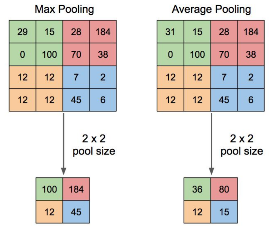
Image Flattening
Once the pooling is done the output needs to be converted to a tabular structure that can be used by an artificial neural network to perform the classification. Note the number of the dense layer as well as the number of neurons can vary depending on the problem statement. Also often a drop out layer is added to prevent overfitting of the algorithm. Dropouts ignore few of the activation maps while training the data however use all activation maps during the testing phase. It prevents overfitting by reducing the correlation between neurons.
Step by step implementation of Natural image processing
- I suggest you to use python 3 because some libraries do not support in python2. You can upgrade or install python 3 separately)
- sudo apt install python3-pip
- Install Jupyter notebook (pip install notebook)
- Install required libraries for the project
- numpy (pip install numpy)
- pandas (pip install pandas)
- matplotlib (pip install matplotlib)
- tensorflow (pip install tensorflow)
- skelton (pip install -U scikit-learn scipy matplotlib)
- seaborn (pip install seaborn)
- Open your terminal and go your project directory where you have all your project dataset images and type “jupyter notebook” and press enter.
- First import all the required library package to the project
import numpy as np #linear algebra
import pandas as pd # CSV file I/O (e.g od.read_csv)
import os
import matplotlib.pyplot as plt
import cv2
import tensorflow

path = 'natural_images'
labels = os.listdir(path)
print(labels)
6. Let’s print the image class names as an array
labels = os.listdir('E:/data/dataset/')
print(labels)
#---Output---
#['airplane', 'car', 'cat', 'dog', 'flower', 'fruit', 'motorbike', 'person']
7. Now we can create a for loop to display 5 images from each class
num = []
for label in labels:
images_path = path+'/{0}/'.format(label)
folder_data = os.listdir(images_path)
k = 0
print('\n', label.upper())
for img_path in folder_data:
if k < 5 :
display(Image(images_path+img_path))
k = k+1
num.append(k)
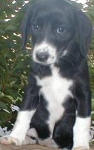
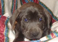
print('There are',k, ' images in', label, 'class')AIRPLANE

There are 727  images in airplane class

 CAT

There are 885  images in cat class

 PERSON


There are 986  images in person class

 DOG
There are 702  images in dog class

8.Now let's plot a diagram to see how may images available on each classes then we can analyse it easily.
x_data = []
y_data = []

for label in labels:
    path = 'datast/{0}/'.format(label)
    folder_data = os.listdir(path)
    for image_path in folder_data:
        image = cv2.imread(path+image_path)
        image_resized = cv2.resize(image, (64,64))
        x_data.append(np.array(image_resized))
        y_data.append(label)
You can buy the project with all the related code files and dataset in one step
Buy my productReferences
Das, A. (2021). Convolution Neural Network for Image Processing — Using Keras. [online] Medium. Available at: https://towardsdatascience.com/convolution-neural-network-for-image-processing-using-keras-dc3429056306.
Saha, S. (2018). A Comprehensive Guide to Convolutional Neural Networks — the ELI5 way. [online] Towards Data Science. Available at: https://towardsdatascience.com/a-comprehensive-guide-to-convolutional-neural-networks-the-eli5-way-3bd2b1164a53.
Image features. (n.d.). [online] Available at: http://morpheo.inrialpes.fr/~Boyer/Teaching/Mosig/feature.pdf.
Stanford Univeristy (2018). Introduction to Convolutional Neural Networks. [online] Available at: https://web.stanford.edu/class/cs231a/lectures/intro_cnn.pdf.
Visin, V.D., Francesco (2016). English: Animation of a variation of the convolution operation. Blue maps are inputs, and cyan maps are outputs. [online] Wikimedia Commons. Available at: https://commons.wikimedia.org/wiki/File:Convolution_arithmetic_-_Same_padding_no_strides.gif [Accessed 20 Aug. 2020].
Bonner, A. (2019). The Complete Beginner’s Guide to Deep Learning: Convolutional Neural Networks. [online] Medium. Available at: https://towardsdatascience.com/wtf-is-image-classification-8e78a8235acb.
check out how to find colour picker on your chrome browser
One thought on “Natural Image Processing Using CNN (Python)”